Chapter 4: Spatial Data Models

A set of rules based on mathematical formulation to represent and visualize geospatial data on a computer screen is called a data model. In GIS environment, these models are divided into two main categories, i.e., Raster Data Model and Vector Data Model. Both models have their own advantages and disadvantages. Based on their characteristics, these models are used to display different type of data.

4.1 Raster Data Model

The geospatial data is represented as a series of equal-sized cells using a grid pattern. These cells are usually square in shape and evenly distributed in “x, y” space. Digital photographic data or images such as satellite imageries or aerial photographs are examples of raster data. Each cell of the image is called pixel (picture element) and holds only one value usually representing the reflectance from the targeted object. The pixel size or the number of pixels determine the sharpness of the image and represent its spatial resolution. The smaller the pixel size, the better the spatial resolution. The entire image is represented as a series of pixels, and no data gaps are found in raster data model making it best suited to represent continuous data such as slope, soil moisture, and digital elevation model (DEM). Since each pixel has a value to store, and the pixels have wall-to-wall coverage of the entire image, the data volume of raster data is usually very high making it slower to display. A better-quality graphic card may be required to display larger datasets. The display size of each pixel will keep on increasing with the zooming level to the point that each data pixel becomes visible; thus, raster data model has a zooming limitation, and the objects may not be recognisable beyond the zooming limit. The pixel size of a raster data also induces errors in the size measurements of an object. The errors in size (volume or length) measurements will be reduced by reducing the pixel size. Similarly, the pixel size of a raster data imposes limitations on its location accuracy and thus rater data usually have limited location accuracy. If the pixel size is reduced to half, the number of pixels in the data will increase four times. Though reducing pixel size will improve image sharpness, measurement, and positional accuracies, it will also increase data volume. Thus, a balance should be achieved between the pixel size and the data volume.

The biggest limitation of a raster data is that it can only have three fields (OID, Value, Count) in its attribute table. These fields can only hold numerical values, usually integer values. The first field is represented by a primary key or unique identification number. The “value” field represents the pixel value, and the last field “count” represents the number of pixels having the same pixel value. The “value” field is mainly used to classify the raster data into various classes. In some cases, the attribute table of a raster data cannot be displayed especially if it represents a continuous data unless it is built. Some software like ArcMap provides tools like “Build Raster Attribute Table” for this purpose. However, the tool will only work on a single band raster data and may not work on a composite raster image. Since raster data volume is usually high and requires better computer resources for its processing, it is advisable to convert it into vector data before processing it. However, some analysis functions can only be applied on raster data and cannot be implemented in vector data. Raster data must be classified into different classes before converting it into vector data.

The raster data models are also known as field-based models. Data for such models is collected directly through aerial photographs or satellite images. Mathematical and geostatistical methods such as interpolations, sampling, or reclassification can also be used to generate data for field-based models. Digital Elevation Model (DEM), weather maps, and heat maps are examples of raster data generated through geostatistical methods where spot data or contour information is used to generate raster/field base data. Spatial phenomena of these data models vary continuously without having specific boundaries.

4.2 Vector Data Model

Vector data is represented in the form of coordinates. These coordinates represent the spatial location and may also be the size or boundary of an object. There are three types of objects in a vector data model, i.e., point, line, or polygon. Point is a dimensionless object representing the location of a feature which is too small to show as a line of polygon at the display scale of the map. A line is a set of points which is used to represent linear features such as roads too narrow to be displayed as an area at the display map scale. Every line will have a starting point, an end point, and intermediate points. Each point on a line is expressed by a set of coordinates. The start and end points of a line are called nodes whereas the intermediate points which also define the shape of the line are called its vertices. Thus, a line may not necessarily be a straight line but could be a combination of several connected straight lines or other linear geometrical shapes like curves. These lines may also be referred as polylines. Similarly, polygon is a combination of connected lines or polylines forming a closed geometry to represent an area of the feature. The starting and end node of a polygon is the same point. Every polygon has an interior region which may enclose another polygon. Adjacent polygons may share their boundaries.

Since the data is recorded in form of coordinates representing a point, line, or polygon, it is only recorded where it is necessary to record. Thus, the data volume of a vector data model is much less as compared with the raster data model. Smaller data volume of vector data makes it faster to display and manipulate, requiring less computer power. The vector data does not get pixelated by zooming. Thus, a map having vector data does not have any zooming limit. The recording of data using coordinates allows accurate measurements of location, length, and area of a feature. However, data capturing scale may impose some restrictions. Similarly, the feature boundaries are very well defined in a vector data model. The vector data models allow users to add as many fields in the attribute table as required without any restrictions of the data format. These fields can easily be updated and can also be joined or related with external tables. The printing cost of maps created using vector data models is much lower than the maps created using raster data models. The vector data can easily be displayed on top of raster data, but raster data cannot be displayed over vector data as it will obstruct the vector data.

The vector base models are also known as object-based models where each object has a specific boundary or dimensions. The data for object-based models is collected through traditional surveying techniques, on-screen digitization, or through interpretation of raster data such as aerial photographs.

The vector data model is further divided into two sub-models.

4.2.1 The Spaghetti Vector Model

Spaghettini data model is the earliest data model developed to represent linear features with each line having its explicit starting and ending points (nodes). Each line is recorded and represented separately. The shared boundary of adjacent polygons may be recorded or represented twice and may not completely overlap. The spaghetti is simple and efficient for data display and plotting. However, it is a relatively unstructured way of representing vector data. The missing feature connectivity information can lead to analysis errors. There may be breaks or overlaps for connecting linear features. Similarly, polygons may not form a closed region and thus the area of a polygon feature cannot be calculated. Thus, the spaghetti model offers very limited spatial analysis in GIS environment. In certain situations, network analysis may not even be possible using spaghetti data model as feature’s topology is not stored. Performing spatial analysis or network analysis may lead to errors in the results as features may not connect when they should. The data should be cleaned, and topological errors should be resolved before performing such analysis.

4.2.2 Topological Vector Models

The limitations of spaghetti models for spatial analysis were resolved through topological data model which greatly improved the speed and accuracy of spatial analysis in GIS environment. This was achieved through strictly enforcing the connectivity and adjacency information. The spatial relationship between similar features is strictly maintained and enforced. This relationship is usually recorded separately from the coordinate information and hence, stretching, bending, or zooming has no effect on the topological information. There is no line or polygon boundary overlap in topological model. The intersecting lines have a node expressing the intersection. Missing node on the crossing lines will indicate that the lines are not coplanar and thus do not intersect and should be treated separately while performing spatial or network analysis. The nodes on the lines may also be used to store to-from information to facilitate linear referencing.

Similarly, overlapping polygon boundary will have only one line segment representing the shared boundary of adjacent polygons. However, non-coplanar polygons will not have shared boundary. Like line feature, nodes are placed at the start and end of the shared boundary of coplanar adjacent polygons.

Topological vector data models allow users to perform several geospatial operations and are thus useful for spatial analysis. However, data must be clean to rectify topological errors. Different GIS software may use different approaches and data structures to store topology. Some software allows users to construct topological relationship when needed to simplify data structures, while others may maintain topological relationship in their data. The computational cost of topological data model is generally high as compared with the spaghetti model. Topological models also require more efforts to create a cleaner data, free from topological errors; however, GIS software generally provide tools to assist in creating cleaner data for topological model. Regardless of the more computational power and efforts required for topological models, it offers much greater benefits in analytical data capabilities.

4.3 Triangulated Irregular Networks (TIN), A Vector Representation of Surface

A vector representation of surface data is typically used to show terrain heights. The location of each point in the dataset is shown using three points in x, y, z domain. The point can be randomly distributed in space but connected in a way to form smallest possible triangles. Each point in the dataset may represent a vertex of one triangle or multiple triangles. Thus, the neighbouring triangles may share their vertices; however, the lines connecting vertices forming edges of different triangles must not cross each other. Convergent circles using three points are drawn and a triangle is drawn only if the convergent circle does not contain any other point in the dataset. This arrangement forms an irregular network of triangles where facet of each triangle represent terrain surface. There could be several mathematical approaches to form such a network of triangles; however, the resultant dataset is much more complicated than a raster data model. TIN data models may be complex but being a vector representation, it can be efficiently displayed and require less data storage. The built-in topological relationship within TIN also makes it suitable for geospatial analysis. Thus, TIN is an efficient alternative of representing Digital Elevation Model (DEM). TIN uses variable data density approach and preserves data points while representing terrain elevations. Thus, TIN can be used to describe a surface at different levels of resolution. Smaller triangles can be used to represent areas with high frequency of elevation changes. Thus, TIN can efficiently show abrupt elevation changes which may be a limitation for raster data representation of DEM; however, it is not suitable for representing large or irregular areas. It might also offer limited area visualization.

4.4 A Comparison of Raster and Vector Data Models

The geospatial data can be recorded, presented, and analysed using different data models. Each data model has its own advantages and disadvantages. One data model may be best suited for one type of analysis whereas the other models perform better under other conditions. Some geospatial data like DEM can be presented using multiple data models. The user can choose a specific data model to perform GIS analysis. However, GIS data models are interchangeable. A comparison of vector and raster data models is explained in Figure 11 and summarized in Table 4.

These parameters may be considered while making a choice between raster and vector data to be used in a GIS project. Usually, coordinate precision, processing speed, memory requirements, and characteristics are main deciding factors for data format selection. However, some data such as satellite imageries are only available in a specific format leaving no choice for users to choose data model. Ease of data capturing methodologies may also be one of the factors for data format selection, as it is one of the most time-consuming, tedious, and expensive processes which can cost up to 50% of the total project cost. It can be the second most important task after data maintenance in multi-year GIS projects. It is generally agreed that raster data models are best suited for resource mapping and analysis, whereas vector data models facilitate network analysis.

 Table 4: Vector and Raster Data

Vector Data ModelRaster Data ModelVector over Raster
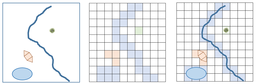
A vector can also be termed as object-based model as features represented by vector models usually have spatial boundaries and can be represented as points, lines, and polygons. However, spatial phenomenon that vary continuously over space without having specific boundaries may be termed as field-based models.

Figure 12: Vector and Raster Data model representation.

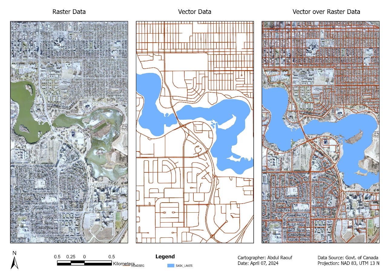
Figure 13: Raster and Vector Data model representation.