Chapter 1: The Earth

The Earth is the fifth largest planet of the solar system which can support life. It is estimated that it is about 4.5 billion years old. Some of the oldest rocks found on the Earth were discovered in Northwestern Canada and Australia. About 70.8% of the Earth is covered with water and the rest is land. At an average distance of about 150 million km from the Sun and with an orbital speed of about 29.8 km/s, it takes about 365.25 mean solar days or one sidereal year to complete its rotation around the Sun. The Earth revolve around its axis of rotation in counterclockwise direction if viewed from celestial north. The Earth’s axis of rotation is tilted by 23.44^o from the perpendicular to the Earth-Sun plan. It takes 23 hours, 56 minutes, and 4 seconds to complete its rotation around its axis of rotation(NASA, 2024).

1.1 The Spherical Earth

According to the Mesopotamian mythology, the Earth was considered as a flat disk with Arctic Circle in the center and Antarctica is a 45.72 m tall wall of ice, around the rim whereas the Sun and the Moon are spheres circulating in circles. However, Aristotle (384 – 322 BC) noted some interesting observation. He observed that the night skies (start configuration) in the northern hemisphere are different than the southern night skies. The length of a shadow increases at noon while travelling away from the equator in north or south direction. He also observed that ships disappear after some time while sailing away from the coast. Most importantly, the Earth cast a circular shadow on the Moon during lunar eclipses. These observations led him to believe that the Earth is not a flat disk but a spherical body of mass. His belief was further strengthened by the fact that horizon increases with altitude. It could be about 5 km for a person of average height (2 m) but can increase up to 36 km if the same person is climbed over a 100 m tall tower. Eratosthenes (276 BC-194 BC) used the observations of changing shadow length at noon while travelling in the north-south direction, to calculate the circumference of the Earth through his famous camel experiment. He dug a deep well in Alexandria, Egypt and noted that the sun rays can reach its bottom at noon. He then travelled south for 50 days to reach Syene (Aswan), Egypt on the Nile River. He dug another well of same depth in Syene and observed that the sun rays at noon are not reaching the depth of the well. He constructed a tower of the same height as the depth of the well and length of its shadow at noon. The height of the tower and its shadow at noon allowed him to calculate the sun angle at noon. These values were used to calculate the circumference of the Earth (Sottosanti, n.d.).
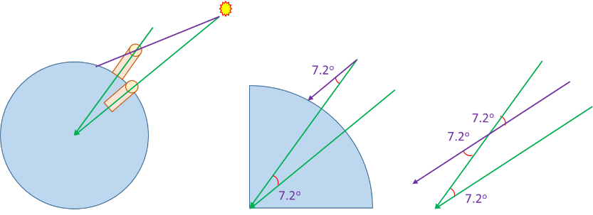Camels travelling 100 stadia/day.
>Travelled for 50 days = 5,000 stadia
7^o12’ = 7.2^o

= 50
50 x 5,000 = 250,000 Stadia
(≈ 46,000 – 48,000 km)
Figure 1: Calculating circumference of the Earth using the camel experiment.
The circumference calculated by Eratosthenes through the camel experiment was very close to the actual circumference of the Earth. The error in the calculation were caused by the fact that the stadia is not a precise unit of distance measurement. The other source of the errors could be the fact that Syene is not precisely south of Alexandria (Sottosanti, n.d.).

1.1.1 Geographical Coordinate System

Once it was decided that the Earth is not a flat disk but a spherical body of mass, a system of lines based on spherical trigonometry was devised to locate a position on the surface of the Earth. This system of imaginary lines is called geographical coordinate system. It is also referred as graticule or a grid. It is composed of circular lines. The lines running in north-south direction are called longitudes or meridians. The lines running in east-west direction are called latitudes or parallels. These lines are drawn using spherical trigonometry with the center at the center of the spherical Earth. The Earth is divided into two hemispheres (northern and southern hemispheres), by a line extending in east-west direction, known as equator. All the lines parallel to equator are called parallels or latitudes. These lines are drawn with an angle from the equator using the concepts of a unit circle. Thus, the latitudes can range from 0 – + 90^o or 0 – 90^o N and 0 – 90^o S, whereas the equator is represented by 0^o. The radius of the equator is the same as the radius of the earth. However, the radius of all other latitudes is less than the radius of the earth and keeps on decreasing depending upon their distance from the center of the Earth. These circles are called small circles.

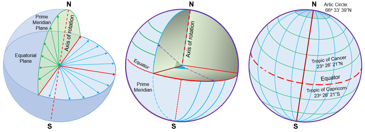
Figure 2: Geographical Coordinates
If the Earth is considered as a perfect sphere, each parallel is equally spaced along a meridian in north-south direction. This spacing can be used to define units of distance (NIST, 2021).
A nautical mile = 1 min of latitude spacing along any meridian
1 meter = one ten-millionth of the distance along a meridian from equator to pole
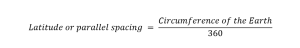
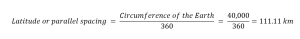
If circumference of the circular Earth is known, the distance between two consecutive latitudes (latitude spacing per degree of latitudes) is given by:

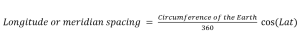
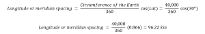
Similarly, north-south circular lines can also be drawn on the Earth. The radius of these circles is the same as the radius of the Earth and thus these circles are called great circles. These lines are called meridians or longitudes. All longitudes converge at the North and the South poles. Thus, the spacing between the longitudes is maximum at the equator and keep on decreasing moving away from the equator. Since all longitudes (meridians) converge at poles, the spacing between longitudes is zero at poles. If circumference of the circular Earth is known, the distance between two consecutive longitudes (longitude spacing per degree of longitude) at a given latitude is given by:

A north-south reference line (half circle) for the longitudes is called prime meridian. The longitude value of the prime meridian is 0^o. A north-south line passing through Greenwich is the agreed location of the prime meridian. The longitudes can range from 0^o to + 180^o or 0 – 180^oE and 0 – 180^oW.
The opposite side of this half circle is called International Date Line (IDL). Since the axis of rotation of the Earth is a line joining the North and South poles passing though the center of the Earth, the longitudes can be used to define time zones of the Earth. A longitude difference of 15^o at equator can be translated as an hour time difference between the two points. All the areas east of the prime meridian will be in advance of the Greenwich Time, and all the areas west of the prime meridian will be behind Greenwich Time. Starting from the prime meridian going east, these are 180^o to the IDL. Thus, the time just east of IDL will be 12 hours ahead of the Greenwich Time. Similarly, the time just west of the IDL will be 12 hours behind the Greenwich Time. Thus, east side of the IDL will have a date one day ahead of its west side. Thus, IDL functions as a line of demarcation separating two consecutive calendar dates. However, it does not have any internal legal status, and regional countries can choose to be on either side of IDL. For this reason, IDL zigzags around political borders because of administrative and financial purposes so that the countries and region across the line can have the same calendar date. It can change because of the changing geopolitical situation and on the request of the regional countries. The recent change in the IDL was requested by Samoan Islands and Tokelau (a territory of New Zealand) in 2011.

1.1.1.1 Example 1: Parallel spacing per degree

Calculate spacing between two consecutive latitudes if the circumference of the Earth is 40,000 km.
>Given: Earth’s circumference = 40,000 km

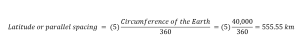
1.1.1.2 Example 2: Parallel spacing

Calculate spacing between 20^o and 25^o latitudes if the circumference of the Earth is 40,000 km.
Given: Earth’s circumference = 40,000 km
Latitude difference = 25^o – 20^o = 5^o

1.1.1.3 Example 3: Longitude spacing per degree at 30o latitude.

Calculate spacing between two consecutive longitudes at 30^o latitude if the circumference of the Earth is 40,000 km.
Given: Earth’s circumference = 40,000 km
Latitude = 30^o

1.1.1.4 Example 4: Longitude spacing at 30o latitude.

Calculate spacing between 20^o and 25^o longitudes at 30^o latitude if the circumference of the Earth is 40,000 km.
Given: Earth’s circumference = 40,000 km
Latitude = 30^o
Longitude Difference = 25^o – 20^o = 5^o
Latitudeorparallelspacing=(5)CircumferenceoftheEarth360cos(Lat)
Longitudeormeridianspacing=540,0003600.866=481.12km

1.2 Earth as Ellipsoid

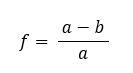
The earth was considered as a perfect sphere until 1060s when Isaac Newton, while working on Laws of motion and the law of gravity, proposed that the shape of the Earth is not spherical but elliptical. The polar radius of the Earth is smaller than its equatorial radius. However, this difference is only about 21.4 km (NOAA, 2023). Thus, the Earth’s minor axis is only about 0.33% smaller than its major axis. That is why it still looks spherical from its vantage point. Latest satellite technologies have revealed that the Earth is an imperfect ellipsoid, and its shape is continuously changing because of the daily tidal effect, drift of tectonic plates, and melting of permafrost. The shape of the Earth can also change because of earthquakes, volcanic eruptions, or meteor strikes. Newton also suggested that the Earth is flatter at the poles and thus it rotates around its minor axis. If “a” and “b” are radius of its minor and major axis, the flattening of the Earth is given by:

Mathematical value of “f” is very small. Thus, inverse flatting  is usually used in the literature to describe the shape of the Earth. An elliptical shape of the Earth has its effect on the parallel spacing; thus, the location of the latitudes is slightly different in spherical and elliptical models of the Earth. This difference increases symmetrically from equator to the pole and is maximum at 45^o latitude. The difference starts decreasing symmetrically above 45^oN and below 45^oS. The location of the poles and the equator remains same in the two models. The spherical model of the Earth is usually called geocentric model whereas the elliptical model is called geodetic model.
Since the Earth is an imperfect ellipsoid, different geocentric and geodetic models are used to represent the surface of the Earth in different parts of the Earth. There is possibility that one model can represent the surface of Earth in one area but may not represent the surface of other areas. A reference surface with a set of reference point for the geographic coordinate system to represent the Earth’s surface is called DATUM or geodetic datum. Change in datum can cause the same point to be shifted by several meters. Thus, one should choose the right datum to map a specific area, country, or a region. The North American Datum of 1983 (NAD 83) is currently used for the United States, Canada, Mexico, and Central America and is based on a geocentric origin and the Geodetic Reference System 1980 (GRS80). The World Geodetic System of 1984 (WGS 84) is a global reference system which is being used by Global Navigation Satellite System (GNSS). The WGS 84 was developed using Doppler satellite surveying techniques.
As we know, the surface of the Earth is not smooth. Top of Mt. Everest is the highest point on the surface of the Earth whereas bottom of the Mariana Trench is the deepest point. A reference to the elevation variations is also required to determine an accurate location of any point on the surface of the Earth. A vertical datum or GEOID as reference surface is introduced to record elevation or height information of any given point. The information derived from the Mean Sea Level (MSL) has been used to develop vertical datum or GEOID. MSL is an average of all low and high tides at a particular point over one Metonic cycle (a 19-year cycle where the Moon returns to the same place). Several tidal gauges are used to record tidal variation to extract MSL. With the advancements in satellite and surveying technologies, GEOID is now defined as a surface of equal gravity and can be different from MSL. Natural Resources Canada (NRCan) has released the latest Canadian Geodetic Vertical Datum in 2013 and is called CGVD2013. The CGVD2013 is compatible with GNSS and is a new reference for elevations across Canada.
The study of the ever-changing shape of the Earth and its gravitational field is called “Geodesy”. Knowledge of Geodesy can help to precisely locate any point of the surface of the Earth.

1.3 Representation of the Earth

One of the most accurate methods of representing the Earth is a globe as it is spherical in shape and can closely resemble the Earth. Thus, all countries and continents can be shown accurately without a noticeable distortion. Other geometric properties such as area, direction, distance, and shape can be preserved. The scale remains the same everywhere on the globe. However, the globe has some limitation when representing the Earth. Some of these limitations are as given below:
Globes cannot display the entire Earth at the same time. At any given time, only a hemisphere is visible to the globe user/reader. Globes can only be constructed at a limited scale. A 550m diameter globe would be required to represent the Earth at a scale of 1:24,000. Areas of countries and continents would be difficult to measure because of the spherical nature of the globe. Bigger globes are not only difficult to construct but also difficult to transport and thus have limited practical value. However, they offer great visual representation of the Earth.
Two-dimensional maps can also be used to represent the Earth or a portion of it. However, the three-dimensional surface of the Earth needs to be transformed into two-dimensional map surface. It is usually achieved by projecting 3D globe onto to 2D map. Different projection systems can be designed and developed to create 2D maps. However, a virtual light source, a generating globe, and a developable surface are three essentials of every projection system. Distortion occurs while transforming location from the generating globe to the developable surface. Thus, every map has some distortion. Different areas on the map may have different level of distortion. The map distortion can be represented either by Tissot’s indicatrix or by scale factor.

Tissot’s indicatrix is a graphical tool to show map distortion in which a grid of regularly spaced circles on a generating globe are shown as ellipsis or circles of varying sizes on the map. The shape and size of these ellipsis or circles indicate the map distortion trends while quantifying the value of distortion. Though Tissot’s indicatrix may be visually appealing to show map distortion, they may obscure the important map features and the resultant map may be overcrowded.
Scale factor is a mathematical ratio of the actual scale to the principal scale. Mathematically it is written as:
ScaleFactorSF=ActualScalePrincipalScale
The actual scale is the scale of the map, and the principal scale is the scale of the generating globe. A scale factor of “1” means no distortion, whereas a scale factor other than “1” represents distortion. Thus, the scale factor should be equal to “1” for large-scale maps to avoid map distortion. A projection system with a scale factor close to “1” is highly desirable.
The map projection family can have the following members depending upon the geometric distortion, the nature of the development surface, and the location of the virtual light source. Mostly, a combinational use of the developable surface and the location of the virtual light source can determine the characteristics of the projection system. An orthographic planner projection system will use a virtual light source placed at an infinite distance from the generating globe to project it on a planner surface. This projection system can preserve the shape of countries and continents. A stereographic planner projection system is a planner system which has its virtual light source at the antipodal point of the generating globe. Such a projection system can be used to preserve angles (directions). Similarly, if the light source is placed at the center of the generating globe to project it on a planner system, it will be a gnomonic planner system which can preserve distance. The cylindrical projection system has only two possibilities for placement of the virtual light source. If the light source is placed at the center of the generating globe, it is a central cylindrical projection system. If the light source is placed at infinity, it is an equal area cylindrical projection system. There is only one possible conic system as the light source can only be placed in the center of the generating globe. It is called a central conic projection system. All the six projection systems discussed above are shown in Figure 3.

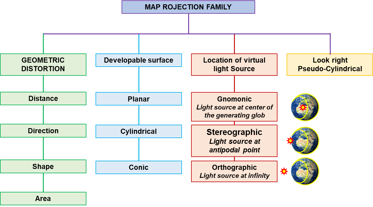
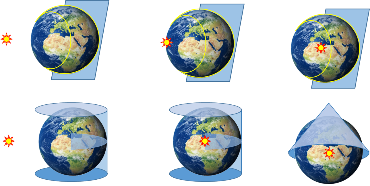
Figure 3: Map projection families

The orientation of the developable surface and its contact with the generating globe also determine the characteristics of the projection system. The tangent case is referred to a situation when the developable surface has minimum contact with the generating globe. It will be point of contact for planner system and a line contact for cylindrical or conic systems. The scale factor will be 1 at the point or line of contact and will keep on increasing away from the contact point or line. The secant case is referred to the situation when the developable surface slices through the generating globe. Thus, a planner surface will form a circle while slicing through the generating globe, whereas cylindrical and conic systems will form two circles. The scale factor will be 1 on the circle lines. It will decrease inward and will increase outward of the circle. The change in the scale factor in the secant cases of the three projection systems is shown in Figure 4.

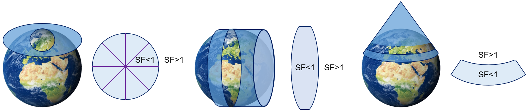
Figure 4: Change of scale factor in secant cases of three projection systems.

Secant case of cylindrical projection system is best suited for world maps of the tropics and is one the most common projection systems used all over the world, whereas secant case of cylindrical projection system is best suited for countries/states of mid latitudes such as east west elongated sates of USA and Australia.

1.4 Map Projection Systems used in Canada.

Canada with its total area of over 9.9 Mkm² is a country spreading from coast to coast to coast. Its 10 provinces and three territories use different projection systems for mapping purpose. However, UTM, LCC and UPS are commonly used projection systems in Canada.

1.4.1 Universal Transverse Mercator (UTM) Projection System

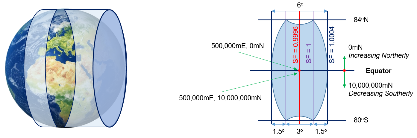
Universal Transverse Mercator (UTM) is one of the commonly used projection systems all over the world. It is a secant case of a cylindrical project system where the cylindrical developable surface is oriented in east-west direction, thus the lines of tangency specifying an area to be mapped, are oriented in north-south direction. These mapping areas are called UTM zones. Each UTM zone is 6^o wide at the equator and keep on decreasing in the north-south direction. In total, 60 north south UTM zones are required to cover the entire globe however, the zones from 80^oS to 84^oN. Zone 1 starts from the International Date Line. The number keeps on increasing eastward from the International Date Line. Canada is covered by UTM zone number 7 to 22. The width of each UTM zone is purposely kept smaller to reduce the distortion caused by the projection system. Thus, scale factor within a UTM zone varies from 0.9996 to 1.0004. The central straight north-south line of each UTM zone is called central meridian and is a reference line for coordinate measurements of each zone. False coordinate also called projected coordinates are used for each zone and are described with the units of length, typically meters. Each UTM is divided in to two subzones for mathematical simplicity. Thus, each zone has its north subzone and south subzone. The assigned false coordinates (projected coordinates) are assigned differently for each subzone. The intersection of the central meridian and the equator for the north zone are 500,000mE and 0mN, however, coordinates the same point of the south zone are 500,000mE and 10,000,000mN. The UTM projection system and its zone is explained in figure 5. If a region is not completed covered within one UTM zone, its edge meridians of a UTM zone can be shifted to accommodate the entire area of the region. For example, Saskatchewan is not completely covered within zone 13, and is partially covered in zone 12 and 14 but the edge meridians of zone 13 are shifted to facilitate one UTM zone mapping for Saskatchewan. Ontario is covered in multiple UTM zones.

Figure 5: UTM Zone

1.4.2 Lambert Conformal Conic (LCC) Projection system

Lambert Conformal Conic (LCC) is a projection system used for cartographic boundary files, digital boundary files, road network files, the Spatial Data Infrastructure, and representative points in Canada. It is also used for censuses mapping in Canada. LCC is a secant case of a conic projection System. The apex conic resides over the North Pole and thus provide a good directional and shape relationships for mid-latitude regions. Lines of tangency for LCC used in Canada are placed at 49°N and 77°N. These tangency lines for edge or standard parallels for mapping in Canada. The scale factor is 1 at these lines and keeps on deceasing inward. It is minimum at 63°N which is the central parallel of the projection system. The central meridian for a Canadian LCC is placed at 91°52’W. The central meridian is a straight line, and the projection system is symmetrical on both sides of the central meridian. LCC can conform area more accurately as compared with other projection systems as all meridians intersect parallels at 90^o. The origin of the coordinate system is placed on a parallel south of the bottom standard parallel to ensure that all the false coordinates are positive. These false coordinates are expressed in linear units of meters. Different Canadian provinces used slightly different parameters of LCC to meet their mapping requirements. For example, British Columbia (BC) use 50°N and 58.3°N as standard parallels. The central meridian is placed at 120°W. Latitude of projection origin is placed at 45°N. The false coordinates of the point intersecting the central meridian and the latitude of projection origin are 1,000,000mE and 0mN. It is based on NAD83 datum and the GRS80 ellipsoid. A brief description of the Canadian and BC LCC is given in figure 6.

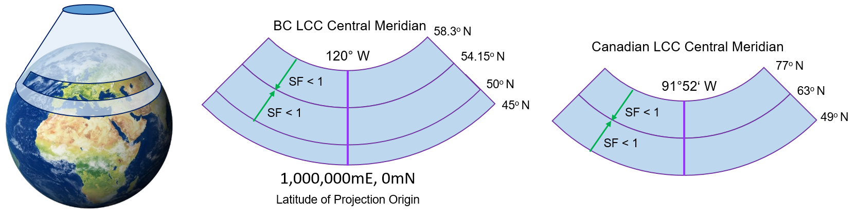
Figure 6: LCC Projection system used in Canada.

1.4.3 Universal Polar Stereographic (UPS) Projection System

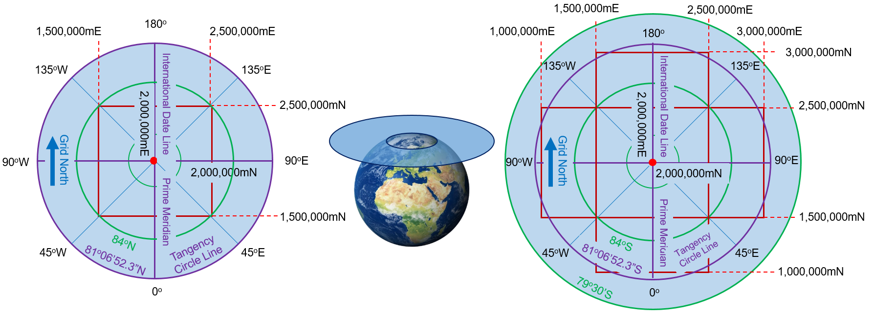
Polar Regions of the world are best covered by the Universal Polar Stereographic (UPS) Projection System which is a secant case of a polar stereographic projection system. The virtual light source is placed at the antipodal point of the generating globe and the planner surface slices through the globe at 84^oN to cover the northern polar region or at 79^o30’S to cover the southern polar region. The line of tangency is placed at 81^o06’52.3” N (81.114528N) or 81^o06’52.3”S (81.114528 S) depending upon the region to be covered. The scale factor decreases inward from the circular line of tangency and is minimum at the pole which is also the center of the map. The minimum scale factor is 0.994. Linear units of meter are used to specify the coordinates of UPS projection system. The false coordinates assigned to either pole is 2,000,000mE and 2,000,000mN. The meridians are straight lines extending outward originating from the center of the map or either of the poles. The parallels are circles around the poles. All the meridians intersect with parallels at right angle. Thus, it is a conformal projection system preserving direction and area. Limited coverage of up to the hemisphere is one of the limitations of UPS, however, it is designed to cover higher latitudes of the world. The UPS, when used in conjunction with UTM can cover the entire world. A brief description of UPS zones is given in Figure 7.

Figure 7: UPS North Zone

1.4.4 EPSG Codes

European Petroleum Survey Group (EPSG) was an informal scientific organization who took an initiative to standardize, improve and share spatial data between members of the organization by creating a database and a public registry of geodetic datums, spatial reference systems, Earth ellipsoids, coordinate transformations and related units of measurement. Each entity is assigned an EPSG code between 1024 and 32767. The metadata of each code conforms to ISO 19115:2019 standards which is dedicated standard for Geographic information – Metadata.

The dataset was made public in 1993. The ESPG was reformed or rebranded as the International Association of Oil and Gas Producers (IOGP). It is the duty of the IOGP Geomatics Committee’s Geodesy Subcommittee to maintain and distribute the EPSG Dataset (IOGP, 2022). Most geographic information systems (GIS) and GIS libraries use EPSG codes as Spatial Reference System Identifiers (SRIDs) and EPSG definition data for identifying coordinate reference systems, projections, and performing transformations between these systems, while some also support SRIDs issued by other organizations.

The EPSG Dataset can be obtained either through:

• A web-based delivery platform https://epsg.org with a graphic user interface (GUI) and an application programming interface (API). Possible to obtain WKT (ISO 19162) or GML files.
• A MS Access database, derived from the online registry.
• A SQL script able users to create an Oracle, MySQL or PostgreSQL database and populate it with the EPSG Dataset.

IOGP has also published a guidance document EPSG Dataset user. It is a multi-part document.

• Part 0, Quick Start Guide: It gives a basic overview of the Dataset and its use.
• Part 1, Using the Dataset: This document sets out detailed information about the Dataset and its content, maintenance, and terms of use.
• Part 2, Formulas: This pat provides a detailed explanation of formulas necessary for executing coordinate conversions and transformations using the coordinate operation methods supported in the EPSG dataset. Geodetic parameters in the Dataset are consistent with these formulas.
• Part 3, Registry Developer Guide: It is primarily intended to assist computer application developers who wish to use the API of the Registry to query and retrieve entities and attributes from the dataset.
• Part 4, Database Developer Guide: It is primarily intended to assist computer application developers who wish to use the Database or its relational data model to query and retrieve entities and attributes from the dataset.

For NAD 83 (CSRS) UTM zone 13N, the code is EPSG 2957. However, the entire UTM zone 13N with NAD 83 is represented by EPSG 26913. An entire list EPSG codes used for different regions of Canada can be found at: https://epsg.io/?q=Canada&page=1. The EPSG 3857 is used by web-based mapping services such as Google and open street maps. EPSG 4326 is a code for WGS 84 and can be sued interchangeably when referring WGS84 as a datum. However, WGS84 traditionally uses latitude-longitude, while EPSG 4326 is defined as longitude-latitude. The swapped coordinates may cause misinterpreting of the area.

1.4.5 Geographic Coordinates vs Projected Coordinates

Both geographic and projected coordinates are important from mapping perspective as both can be used to determine specific location on the surface of the Earth. A brief comparison of the geographic and projected coordinates is given in Table 1:

 Table 1: Geographic and Projected Coordinate Systems

1.5 Map Categories

A map is a 2D representation of a 3D Earth. Depending upon its uses, it can be divided into different categories. Topographic and Thematic Maps are commonly used map categories.

1.5.1 Topographic Maps

As its name suggest, a topographic map is a detailed and quantitative representation of the Earth’s surface. It may include natural features such as ground relief (landforms and terrain), hydrography (lakes and rivers), and forest cover. These maps also include man-made features such as administrative areas, populated areas, transportation routes and facilities (including roads and railways). Topographic maps are suitable for a wide variety of applications, from emergency management, urban planning, surveying, resource development, and tourism etc. (NRCan, 2014).

1.5.2 Thematic Maps

Thematic maps are single-topic maps that showing spatial distribution of specific data themes or phenomena, such as population density, rainfall and precipitation levels, vegetation distribution, and poverty. These maps can be quantitative or qualitative. These maps are very useful for analyzing spatial distribution of phenomena while identifying geographic patterns, trends, and correlation within the geospatial datasets. Thematic maps are generally allied with geo-visualization of the data where properties of features, play important role as compared with their location. Various statistical techniques can be used for creating thematic maps (Dent, Torguson, & Hodler, 2009).

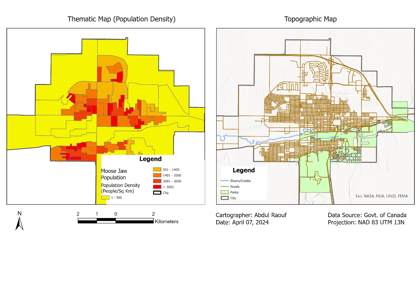
Figure 8: Thematic and Topographic Maps